For today’s blog post, I want to focus our attention on the first Lightboard video: How Volumes work on FlashArray and a discrete benefit to FlashArray’s architecture. If you’re not yet familiar with that, I strongly suggest you read “Re-Thinking What We’ve Known About Storage” first.
Silly Analogy Time!
As many of you know from my presentations, I pride myself on silly analogies to explain concepts. So here’s a silly one that I hope will help to explain a key benefit of our “software defined” volumes.
My wife Deborah (b|t) and I have a chihuahua mix named Sebastian. And like many dog owners, we take way too many of pictures of our dog. So let’s pretend that Deborah and I are both standing next to one another and we each snap photos of the dog on our respective smartphones.
Sebastian wasn’t quite ready for for me, but posed perfectly for Deborah (of course)!
We also have a home NAS. Both Deborah and I have our own volume shares on the NAS and each of our smartphones automatically backs up to each of our respective shares. So once on the NAS, each photo would consume X megabytes per photo, right? That’s what we’re all used to.
Software Saves Space!
Now let’s pretend that instead of a regular consumer NAS, I was lucky enough to have a Pure Storage FlashArray as my home NAS. One of its special super powers is that it deduplicates data, not just within a given volume, but across all volumes across the entire array! So for example, if I have 3 different copies of the same SQL Server 2022 ISO file on the NAS, just in different volumes, FlashArray would dedupe that down to one underneath the covers.
But FlashArray’s dedupe is not just done at the full file level – it goes deeper than that!
So going back to our example, when we each upload our respective photos to our individual backup volumes, commonalities will be detected and deduplicated. Sebastian’s head is turned differently and he’s holding his right paw up in one photo but not the other. Otherwise, the two photos are practically identical.
So instead of having to store two different photos, it can singly store the identical elements of the photo as a “shared” canvas and plus the distinct differences. (If your mind goes to the binary bits and bytes that comprise a digital photo, I’m going to ask you to set that aside and just think about the visual scene that was captured. This is just a silly analogy after all.)
How About Some Numbers?
Let’s say each photo is 10MB each, and 85% of the two photos’ canvas is shared while the remaining 15% is unique to each photo. If we had traditional storage, we’d need 20MB to store both photos. But with deduplication technology, we’d only need to store 11.5MB! That breaks down as 8.5MB (shared: photo 1 & 2) + 1.5MB (unique: photo 1) + 1.5MB (unique: photo 2). That’s a huge amount of space savings, by being able to consolidate duplicate canvases!
Think At Scale
As I mentioned earlier, Deborah and I take TONS of photos of our dog. Most happen to be around our house. And because Sebastian is a jittery little guy, we’ll take a dozen shots just to try to get one good one out of the batch. And if we had data deduplication capabilities on our home NAS, that’d translate to a huge amount of capacity savings that is otherwise wasted storing redundant canvases.
What About the Real World?
Silly analogies aside, what does this look like in the real world? On Pure Storage FlashArray, a single SQL Server database get an average of 3.5:1 data reduction (comprised of data deduplication + compression), but that ratio skyrockets as you persist additional copies of a given database (ex: client federated dbs, non-prod copies on staging, QA, etc. ). If your databases are just a few hundred gigabytes, you might not care. But once you start getting into the terabyte range, the data reduction savings starts to add up FAST.
Wouldn’t you be happy if your 10TB SQL Server database only consumed 2.85TB of actual capacity? I sure would be. Thanks for reading!
For today’s blog post, I want to focus on the subject matter of the first Lightboard video: How Volumes work on FlashArray.
Storage is Simple, Right?
For my many years as a SQL Server database developer and administrator, I always thought rather simplistically of storage. I had a working knowledge of how spinning media worked, and basic SAN & RAID architecture knowledge from a high level. And then flash media came along and I recall learning about its differences and nuances.
But fundamentally, storage still remained a simplistic matter in my mind – it was the physical location to write your data. Frankly, I never thought about how storage and a SAN could offer much much more than simply that.
A Legacy of Spinning Platters
Many of us, myself included, grew up with spinning platters as our primary storage media. Over the early years, engineers have come up with a variety of creative ways to squeeze out better performance. One progression was to move from one single disk to many disks working together collectively in a SAN. That enabled us to stripe or “parallelize” a given workload across many disks rather than just be stuck with the physical performance constraints of a single disk.
Carve It Up
In the above simplified example, we have a SAN with 16 disks. And let’s say that each disk gives us 1,000 IOPs @ 4kb. I have a SQL Server whose workload needs 4,000 IOPs for my data files and 6,000 IOPs for my transaction log. So I would have to create two volumes containing the appropriate number of disks from the SAN to give me the performance characteristics that I require for my workload. (Remember, this is a SIMPLIFIED diagram to illustrate the general point)
Now imagine being a SAN admin trying to have to juggle hundreds of volumes across dozens of attached servers, each with their own performance demands. Not only is that a huge challenge to keep organized, but it’s highly unlikely that every server will have their performance demands met, given the finite number of disks available. What a headache, right?
But what if we were no longer limited by the constraints presented by spinning platters? Can we approach this differently?
Letting Go Of What We Once Knew
One thing that can be a challenge for many technologists, myself especially, is letting go of old practices. Oftentimes those practices were learned a very hard way, so we want to make sure we never have go through whatever rough times again. Even when we’re presented with new technology, we often just stick to the “tried and true” way of doing certain things, because we know it works.
One of things “tried and true” things we can revisit with Pure Storage and FlashArray is the headache of carving up a SAN to get specific performance characteristics for our volumes. When Pure Storage first came to be, they focused solely on all-flash storage. As such, they were not tied to legacy spinning disk paradigms and could dream up new ways of doing things that suited flash storage media.
Abstractions For The Win
On FlashArray, a volume is not a subset or physical allocation of storage media assigned to it. Instead, a volume on FlashArray is just a collection of pointers to wherever the data wound up being landed.
Silly analogy: pretend you’re boarding a plane. On a traditional airline, typically first class boards first and goes to first class, then premium economy passengers go board to their section, then regular economy boards and go to their section, and basic economy finally boards and goes to theirs. But if you were on Southwest Airlines, you can choose your own seat. So you’d board, and simply go wherever you wish (and pretend you report back that you’ve taken a particular seat to an employee). Legacy storage is like that traditional airline where you (data) were limited to sit down in to your respective seat class, because that’s how the airplane was pre-allocated. But on FlashArray, you’re not limited in that way and can simply sit where you like, because you (data) have access to sit anywhere.
Another way of describing it that might resonate is that legacy storage assigned disk storage to a volume and whatever data landed on that volume landed on the corresponding assigned disk. On FlashArray, the data can be landed anywhere on the entire array, and the volume that the data was written to simply stores a pointer to wherever the data wound up on the array.
Fundamental Changes Make a Difference
This key fundamental change in how FlashArray stores your data, opens up a huge realm of other interesting capabilities that were either not possible or much more difficult to accomplish on spinning platters. I like to describe it as software-enhanced storage, because there’s many things we’re doing besides just “writing your data to disk” on the software layer. In fact, we’re not quite writing your raw data to disk… there’s an element of “pre-processing” that takes place. But that’s another blog for another day.
Take 3 Minutes for a Good Laugh
If you want to watch me draw some diagrams on a lightboard that illustrate all of this, then please go watch How Volumes work on FlashArray. It’s only a few minutes long and listening to me on 2x is quite entertaining in of itself. Just be sure to re-watch it to actually listen to the content, because I’m guarantee you’ll be laughing your ass at me chattering at 2x speed. 🙂
I’ll admit this up front – there’s a ton of awesome technologies out there that I’ve had my eye on, learned a little bit about, and have hardly touched since. Docker is one of those technologies… along with Grafana. Well conveniently enough for me, Anthony Nocentino just wrote a blog post on Monitoring with the Pure Storage FlashArray OpenMetrics Exporter. And this monitoring solution uses both. And best of all, it’s actually quite easy to implement – even for a clueless rookie like me!
Recap of Andy Stumbling Along…
Ages ago, I had attended an introductory session or two on Docker, and read some random blogs about it, but otherwise not really messed with it too much beyond a few examples. So I thought I’d just take the quick and dirty route, went into my team lab, and installed Docker Desktop for Windows on a random Windows VM of mine. And while I waited… and waited… and waited for the installation to run, let me go on a slight tangent here.
Tangent – Where To Run Docker From
TL;DR – Docker on Windows is a lousy experience. I expected it to “run okay for a dev box.” Nope, it was worse than that. Run it from a Linux machine if you can – you’ll be much happier.
Slightly longer “why.” Underneath the covers, Docker is essentially Linux. So to run it on Windows, you need to have Hyper-V running, essentially adding virtualization layer. And if you’re silly like me, you’ll do all of this on a Windows machine that’s really a VMware VM… so yay, nested virtualization = mediocre perf!
In my case, after rebooting my VM, Docker failed to start with a lovely “The Virtual Machine Management Service failed to start the virtual machine ‘DockerDesktopVM‘ because one of the Hyper-V components is not running” error. Some quick Google-fu revealed that I had to go into vSphere and on my VM, adjust a CPU setting for Hardware virtualization: Expose hardware assisted virtualization to the guest OS.
Three reboots later, and I finally had Docker for Windows running. Learn from lazy Andy… it would have been faster for me to just spin up a Linux VM and get docker installed and running.
Let’s Monitor a Pure FlashArray!
At this point, I could start with Anthony’s Getting Started instructions. That was super easy at least – Anthony outlined everything that I needed to do.
I did encounter another error after I ran ‘docker-compose up –detach’ for the first time: ‘Error response from daemon: user declined directory sharing‘. That one involved another Docker setting about file sharing. Once I changed that, it errored again, because I failed to restart Docker – doh! At least I didn’t have to reboot my VM again?
So finally I ran ‘docker-compose up –detach’ and stuff started appearing in my terminal – yay! I immediately went to the next step of opening a browser and got a browser error. WHUT?!? I thought something was broken, because Docker was “doing” something. But the reality is that prometheus, grafana, and the exporter, all had to do some stuff before the dashboard was up and available. Several more minutes later, I had a working Grafana and dashboard of my Pure FlashArray – yay!
Take the Time to Try Something New
All of the above took maybe a half hour at most? And a chunk of that was waiting around for stuff to complete, and other time was burned resolving the two errors I encountered. So not a huge time investment to stand up something that is really useful to monitor if you don’t have monitoring tools in place already.
But most importantly, this little experience was gratifying. It felt good to try something new again and to be able to stand this up pretty quickly and fairly painlessly. And if you don’t repeat my mistakes above, you can get your own monitoring operational even faster!
One of the many things I speak about regularly at Pure Storage is using storage-array based snapshots to create crash consistent snapshots of SQL Server data & log files. But what if one of my databases is using In-Memory OLTP?
TL;DR
Can I still take storage-array snapshots and if yes, will I lose data in my memory-optimized tables? What about data inside my non-durable tables?
Yes, you can take storage-array level crash consistent snapshots on FlashArray and data in your memory-optimized tables will remain intact in all volumes cloned from the snapshot.
How Does All Of This Work?
In-Memory OLTP is all about storing your data in RAM. However, there are two different types of table constructs: memory-optimized tables and non-durable tables.
Memory-optimized tables have a secondary copy of their contents stored on disk, but only for the case of server crashes.
Non-durable tables are also memory-optimized tables. However, they differ in that they are defined with their DURABILITY property set to SCHEMA_ONLY. This means the structure of the table is persisted to disk, but never the underlying data.
Because of the need for durability, we can still take storage-array level snapshots that are crash consistent, and use those snapshots for various purposes like dev/test database refreshes. We just would not get the ephemeral data in the non-durable tables, but that’s no different than not getting data in temp tables or table variables.
And remember that crash consistent snapshots differ from application consistent snapshots. Most of us SQL Server professionals are familiar with the latter, that have to go through VSS and stun SQL Server. Crash consistent snapshots do not stun the server though there’s other trade-offs (I ought to just write a blog breaking that difference down, shouldn’t I?).
Have a Demo?
At some point in the future, I’ll make a video recording of me doing this demo, which I’ll post to YouTube and link to here.
I’ve taken the liberty of creating some scripts that will help demonstrate this. This specific example is for two SQL Server instances on VMware, with FlashArray behind the scenes, using vVols. The example database, AdventureWorks_EXT, has the data and log files all on the same vVol for demo simplicity.
1_SETUP – SourceSvr – AdvWrks.sql Restores a copy of AdventureWorks on the SOURCE server. Get a backup file here. Then adds memory-optimized objects and data, using sample code from here.
2_SETUP – TargetSvr – AdvWrks.sql Creates a stub of AdventureWorks on the TARGET server. Was generated from SSMS using ‘Script Database as CREATE’ on the SOURCE server’s copy of AdventureWorks. You can substitute your own instead of running this script.
3_DEMO – SourceSvr – AdvWrks.sql First step of the actual demo, which executes the in-memory OLTP sample code to create some durable and non-durable data.
4_DEMO – PowerShell Snapshots.ps1 Second step of the actual demo, that uses PowerShell to take a crash consistent snapshot of the Source vVol and overlay the Target vVol.
5_DEMO – TargetSvr – AdvWrks.sql Final step of the demo, to query the memory-optimized and non-durable tables on the Target, to see if the data created in ‘3_DEMO – SourceSvr – AdvWrks’ was replicated to the Target server.
One More Caveat
If you also use delayed durability, note that transactions that have not yet been hardened will also not be present in a crash consistent snapshot. It is a trade-off of delayed durability, but is no different than losing a non-hardened transaction with a SQL Server crash/failure.
One of the amazing aspects of my job at Pure Storage, is that I get opportunities to work with new and emerging tech, oftentimes before it is available to the general public. Such is the case with SQL Server 2022, where I got to help test QAT backups for SQL Server 2022.
TL;DR
Using QAT compression for your native SQL Server backups will give you better compression with less CPU overhead, than “legacy” compression. So I get smaller backup files, faster, with less CPU burn. What’s there to not like?
Tell Me More About This Q… A… T… Thing!
So QAT stands for Intel’s Quick Assist Technology, which is a hardware accelerator for compression. It’s actually been around for many years, but most regular folks like myself never got exposed to it, because you need a QAT expansion card in your server to even have access to its powers. And for us SQL Server folks, we had nothing that took advantage of QuickAssist Technology… until now thanks to SQL Server 2022.
In SQL Server 2022, Microsoft has introduced QAT support for Backup Compression. And as I demonstrated in this blog post, your backup files are essentially byte-for-byte copies of your data files (when not using compression or encryption). And I don’t know about you and your databases, but the SQL Server environments I see these days, database sizes continue to grow and grow and grow… so I hope you use compression to save backup time and space!
But I Don’t Have QAT Cards In My SQL Servers
I said earlier that QAT has been around for a number of years, available as expansion cards. But because SQL Server had no hooks to use QAT, I strongly doubt that any of us splurged for QAT cards to be added into our SQL Servers. But there’s two things coming that’ll change all of that…
First, SQL Server 2022 has both QAT hardware support AND QAT software emulation. This means you can leverage QAT goodness WITHOUT a QAT expansion card.
Second, the next generation of Intel server processors will have QAT hardware support built in! So the next time you do a hardware refresh, and you buy the next gen of Intel server CPUs, you’ll have QAT support!
Third, if you cannot get the latest snazzy CPUs in your next hardware refresh, QAT cards are CHEAP. Like, less than $1k, just put it on a corporate charge card cheap.
IMPORTANT – QAT hardware support is an Enterprise Edition feature. But you can use QAT software mode with Standard Edition. And if you stay tuned, you’ll come to find that I’ve become a big fan of QAT software mode.
How’d You Test This Andy?
In my team’s lab, we have some older hardware lying around that I was able to leverage to test this out. Microsoft sent us an Intel 8970 QAT card, which we installed into one of our bare metal SQL Servers, an older Dell R720 with 2x Xeon E5-2697 CPUs and 512GB of RAM.
Database being backed up is a 3.4TB database, with the data spread across 9 data files across 9 data volumes. The data volumes were hosted on a FlashArray and the backup target was a FlashBlade.
To test, I used the above database and executed a bunch of BACKUP commands with different combinations of parameters. I leveraged Nic Cain’s BACKUP Test Harness to generate my T-SQL backup code. If you haven’t used it before, it’ll generate a bunch of permutations of BACKUP commands for you, mixing and matching different parameters and variables. I was particularly pleased that it also included baseline commands like a plain old BACKUP, and a DISK=NUL variant. I did have to make some modifications to the test harness to add in COMPRESSION options: NO_COMPRESSION, MS_XPRESS (i.e. legacy COMPRESSION), and QAT_DEFATE.
Sample BACKUP command used
Tangent: Backup READER & WRITER Threads
So I’ve always known that if you specify more output backup files, that’ll decrease your backup tremendously. But I never quite understood why, until I started this exercise and Anthony Nocentino taught me a bit about BACKUP internals.
In a backup operation, there’s reader threads that are consuming and processing your data, and there are writer threads that’s pushing your data out to your backup target files. If you run a bare bones basic BACKUP command, you get one READER thread and one WRITER thread to do your work. If you add additional DISK = ‘foobar.bak’ parameters, that’ll give you more WRITER threads; 1 per DISK target specified. If you want to get more READER threads, your database has to be split across multiple data VOLUMES (not files or filegroups).
If you were paying attention above, you’ll note that my test database consists of 9 data files across 9 data volumes. I set it up this way because I wanted more READER threads available to me, to help drive the BACKUP harder and faster.
Keep in mind, there’s always a trade-off in SQL Server. In this case, the more threads you’re running, the more CPU you’ll burn. And if you’re doing a bunch of database backups in parallel, or trying to run your backups at the same time as something else CPU heavy (other maintenance tasks, nightly processing, etc.) you may crush your CPU.
Tangent: FlashBlade as a Backup Target
FlashBlade is a scale-out storage array, whose super-power amounts to parallel READ and WRITE of your data. Each chassis has multiple blades and you can stripe your backup files across each of the different blades for amazing throughput. When you look at the sample BACKUP command, you’ll see different destination IP addresses. It is through these multiple Virtual IPs, which go to same appliance, but helps to stripe the backup data across multiple blades in FlashBlade.
Test Results
Legend
Compression Type
Definition
NO_COMPRESSION
No BACKUP compression used at all.
MS_XPRESS
“Legacy” BACKUP compression used.
QAT_DEFLATE (Software)
QAT BACKUP compression – Software emulation mode used
QAT_DEFLATE
QAT BACKUP compression – Hardware offloading used
Baseline: DISK = NUL
BACKUP summary results – DISK = NUL All test results are the average of 3 executions per variable permutation.
Remember, when using DISK = NUL, we’re NOT writing any output – all of the backup file data is essentially thrown away. This is used to test our “best case” scenario, from a READ and BACKUP processing perspective.
It’s interesting to see that without WRITE activity, QAT acceleration did help speed up our BACKUP execution vs legacy compression. And QAT does offer slightly better backup file compression vs legacy compression. But what I find the most impactful is CPU utilization, from both QAT hardware and software modes, is MUCH lower than legacy compression!
Note the Backup Throughput column. We actually hit a bit of a bottleneck here on the READ side, due to an older FibreChannel card in my test server and only having 8x PCIe lanes to read data from my FlashArray. The lab hardware I have access to isn’t cutting edge tech for performance testing, rather older hardware meant more for functionality testing. Moral of this story? Sometimes you I/O subsystem “issues” are because of network OR underlying server infrastructure, like the PCIe lanes and subsequent bandwidth limitations encountered here.
The Best: Files = 8; MTS = 4MB, BufferCount = 100
BACKUP summary results – Files = 8, MTS = 4MB, BufferCount = 100 All test results are the average of 3 executions per variable permutation.
I’m skipping over all of my various permutations to show the best results, which used 8 backup files, MAXTRANSFERSIZE = 2MB, and BUFFERCOUNT = 100.
Much like the DISK = NUL results, QAT yields superior compressed backup file size and CPU utilization. And in this case, Elapsed Time is now inverse – NO_COMPRESSION took the most amount of time, whereas in the DISK = NUL results, NO_COMPRESSION took the least amount of time. Why might that be? Well in the DISK = NUL scenarios, we don’t have to send data over the wire to write a backup target, whereas in this case we did. And using compression of any sort means we will have to send less data out and write less data to our backup target.
Stuck with TDE?
I also TDE encrypted my test database, then re-ran more tests. I found it interesting to see how a TDE database wound up taking more time across the board. And I found it interesting that with TDE + legacy compression, CPU usage was slightly lower but throughput was worse, vs non-TDE + legacy compression.
Parting Thoughts
Of course, the above is just a relatively small set of tests, against a single database. Yet, based on these results and other testing I’ve seen by Glenn Berry, I will admit that I’m VERY excited about SQL Server 2022 bringing QAT to the table to help improve BACKUP performance.
Even if you are stuck with older CPUs and do not have a QAT hardware card to offload to, QAT software mode beats legacy compression across the board.
I do need to test RESTORE next, because your BACKUPs are worthless if they cannot be restored successfully. But alas, that’s for another time and another blog post!
In all of my years working with SQL Server, I never really thought about the actual contents of a SQL Server backup file. Sure, it contains data from a given database, but despite my love of storage engine internals, backup file internals is not something I’ve ever had any interest in looking into.
Until now…
The Premise
This first came up during my onboarding with Pure Storage. Anthony Nocentino (b|t) taught me that a SQL Server backup file is a byte-for-byte copy of your data, as materialized in SQL Server MDF files (assuming no backup compression or backup encryption). And that would make sense – how else would SQL Server store a copy of your data in a backup file? It does not make sense for SQL Server to alter your data when it writes it down to a backup file (again, with NO backup compression/encryption) – that’s a waste of compute and effort.
Well, I had a conversation with someone who was unclear about that assertion. I tried some Google-fu to present some supporting materials, but could not actually find any documentation, official or otherwise, to back it up. So here we are.
Why Do You Even Care?
There’s a bit of Pure Storage related background here, so feel free to skip this section if you don’t care about why I’m writing this.
On FlashArray, we de-duplicate your data behind the scenes across the entire array. So if you had three SQL Servers (Prod, QA, Dev) all attached to a given FlashArray, and each instance had an identical copy of AdventureWorks, it would almost completely dedupe down to one copy on FlashArray.
Along those lines, a single database will have many places where deduplication can also occur within it. Think about how much repetition occurs within a stereotypical dataset. Things like dates, product IDs, product category IDs, etc. are all duplicated throughout a typical dataset, thus ripe for FlashArray to dedupe within your data file too.
But much like the data that resides in each of our databases, there’s a great degree of variability too. You may have a database where practically everything is unique. You may have a database that stores binary data. The list goes on and on. So while we see a certain average deduplication ratio with SQL Server databases, that’s AVERAGE. And often our customers want to know what THEIR database will yield.
And this is where a backup file comes into play.
One trick that Anthony taught me is to provision an empty volume on FlashArray and take a single uncompressed, unencrypted backup of your database and stick the file there. Because the backup file contains a byte-for-byte copy of your data, as materialized in your MDF/NDF files, its dedupe yield will be very close to that of your MDF/NDF files.
Great way to test, huh? Unfortunately the individual I was speaking with was not confident about the underlying byte-for-byte composition of a backup file. So I decided to test, validate, and document it!
Testing Setup
Using SQL Server 2017, I created a simple database with a single table and inserted some data.
Then I created an uncompressed, unencrypted backup file. Finally, I shut down SQL Server’s service and copied the MDF and BAK to another location to begin analysis.
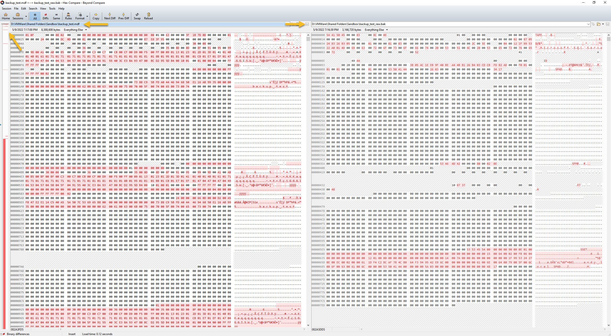
To quickly analyze differences, I found a cool piece of software called Beyond Compare that has a “Hex Compare” feature – perfect for binary file comparison!
To give you a quick overview, the left sidebar shows an overview of the two files, with red lines/blocks to designate some kind of difference in the file. In the example screenshot, the left is the MDF file and the right panel is the backup file. This is the beginning of each file, so you can see that there are some differences present here.
Why Is More Than Half Red?!
However, look closer at the sidebar. The first half has very few differences. But what about that second half that’s ALL RED?
At least that answer is easy. All of those 00’s is simply extra empty space that has been padded at the end of the MDF file. And because it has nothing, it has been omitted from the backup file. I could have truncated the data file first, but I kept this here to illustrate that one’s data file may be larger than the backup file due to this nuance.
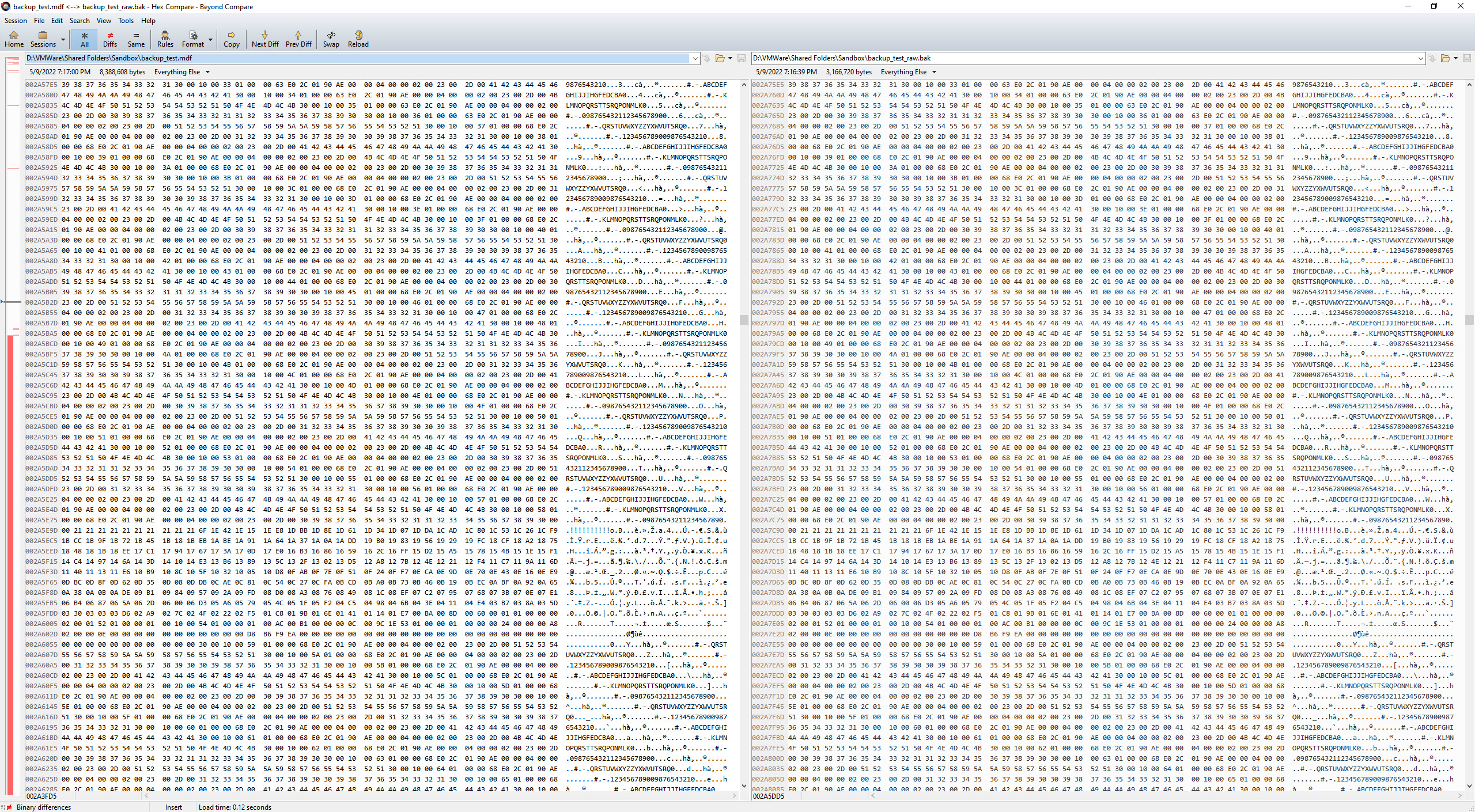
As for the data itself, that’s present in the 2nd quarter of the MDF file or final 3rd of the backup file. And you can see from this screenshot that the backup file is in fact a byte-for-byte copy of the MDF file!
Takeaways
First, I hope that this is enough to prove that data in a database are re-materlized byte-for-byte in a backup file. Sure, there’s some differences in other metadata, but what I care about in this exercise is whether the data itself is identical, which it is.
Second, if you are still in doubt, I’ve published everything to my github here. If you look inside backup_test.sql, you’ll find some extra code in the form of DBCC IND and DBCC PAGE commands. Instead of searching for data, try using DBCC IND and find a different data structure like an IAM page. Then use DBCC PAGE to look at the raw contents and use the hex editor to search for the matching binary data in both the MDF and backup file. I did that myself and found it cool that those underlying supporting pages are also materialized identically.
Third, if you see a hole or gap with this analysis, please let me know in the comments. I did this to learn and validate things for myself, and I definitely want to know if I made a goof somewhere!
Finally, I hope you enjoyed this and stay curious.